JupySQL and chDB
JupySQL is a Python library that lets you run SQL in Jupyter notebooks and the IPython shell. In this guide, we're going to learn how to query data using chDB and JupySQL.
Setup
Let's first create a virtual environment:
And then, we'll install JupySQL, IPython, and Jupyter Lab:
We can use JupySQL in IPython, which we can launch by running:
Or in Jupyter Lab, by running:
If you're using Jupyter Lab, you'll need to create a notebook before following the rest of the guide.
Downloading a dataset
We're going to use one of Jeff Sackmann's tennis_atp dataset, which contains metadata about players and their rankings over time. Let's start by downloading the rankings files:
Configuring chDB and JupySQL
Next, let's import the dbapi module for chDB:
And we'll create a chDB connection.
Any data that we persist will be saved to the atp.chdb directory:
Let's now load the sql magic and create a connection to chDB:
Next, we'll display the display limit so that results of queries won't be truncated:
## Querying data in CSV files
We've downloaded a bunch of files with the atp_rankings prefix.
Let's use the DESCRIBE clause to understand the schema:
We can also write a SELECT query directly against these files to see what the data looks like:
The format of the data is a bit weird.
Let's clean that date up and use the REPLACE clause to return the cleaned up ranking_date:
Importing CSV files into chDB
Now we're going to store the data from these CSV files in a table. The default database doesn't persist data on disk, so we need to create another database first:
And now we're going to create a table called rankings whose schema will be derived from the structure of the data in the CSV files:
Let's do a quick check on the data in our table:
Looks good - the output, as expected, is the same as when querying the CSV files directly.
We're going to follow the same process for the player metadata. This time the data is all in a single CSV file, so let's download that file:
And then create a table called players based on the content of the CSV file.
We'll also clean up the dob field so that its a Date32 type.
In ClickHouse, the
Datetype only supports dates from 1970 onwards. Since thedobcolumn contains dates from before 1970, we'll use theDate32type instead.
Once that's finished running, we can have a look at the data we've ingested:
Querying chDB
Data ingestion is done, now it's time for the fun part - querying the data!
Tennis players receive points based on how well they perform in the tournaments they play. The points for each player over a 52 week rolling period. We're going to write a query that finds the maximum points accumulate by each player along with their ranking at the time:
It's quite interesting that some of the players in this list accumulated a lot of points without being number 1 with that points total.
Saving queries
We can save queries using the --save parameter on the same line as the %%sql magic.
The --no-execute parameter means that query execution will be skipped.
When we run a saved query it will be converted into a Common Table Expression (CTE) before executing. In the following query we compute the maximum points achieved by players when they were ranked 1:
Querying with parameters
We can also use parameters in our queries. Parameters are just normal variables:
And then we can use the {{variable}} syntax in our query.
The following query finds the players who had the least number of days between when they first had a ranking in the top 10 and last had a ranking in the top 10:
Plotting histograms
JupySQL also has limited charting functionality. We can create box plots or histograms.
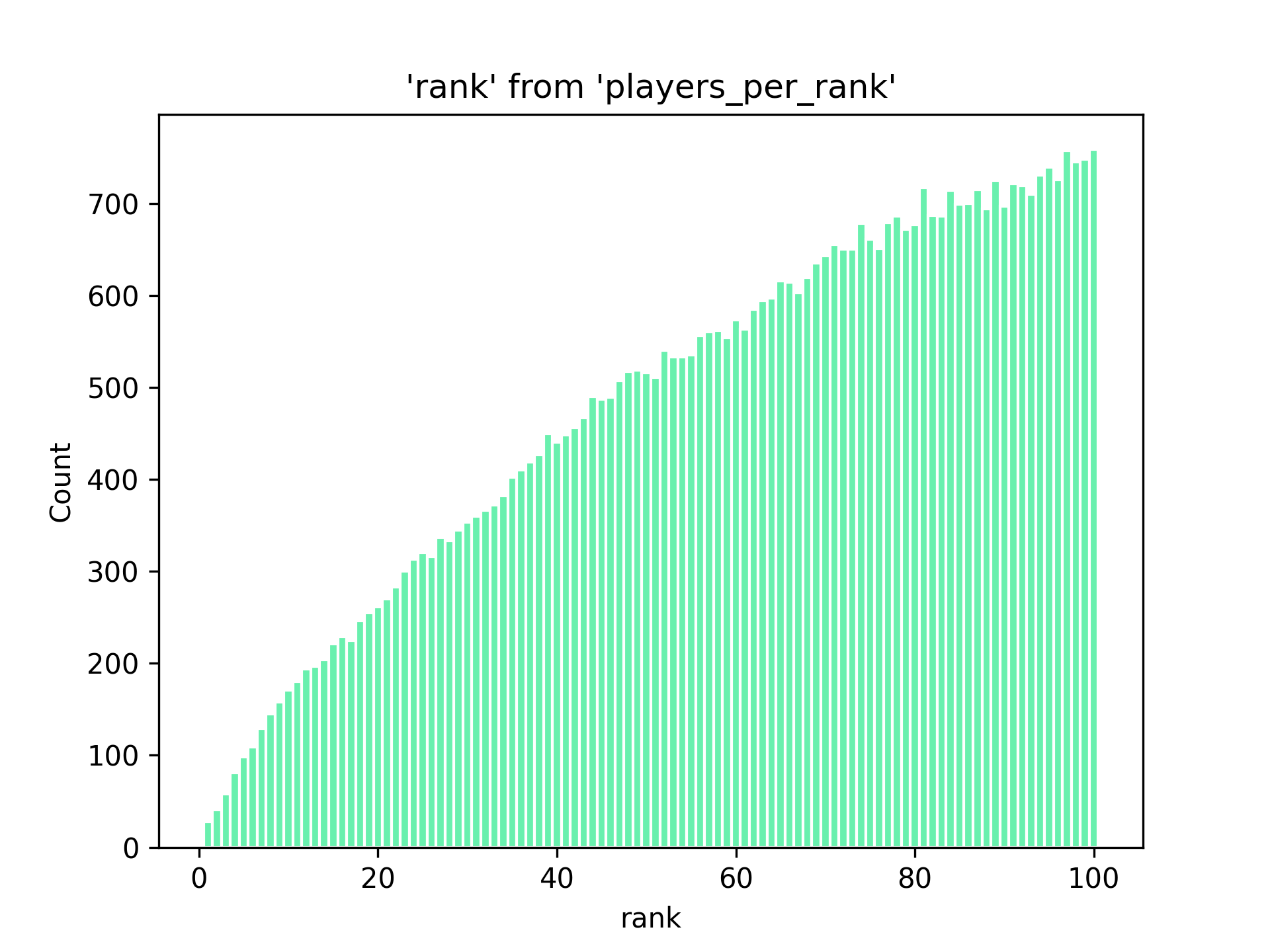
We're going to create a histogram, but first let's write (and save) a query that computes the rankings within the top 100 that each player has achieved. We'll be able to use this to create a histogram that counts how many players achieved each ranking:
We can then create a histogram by running the following:


